How to import shapefiles into Grasshopper using Urbano
In this tutorial, we are going to explore how to import vector and features data from a shapefile into a Grasshopper definition using Urbano plugin. We assume that you already have installed Rhino 6 as well as completed Rhino and Grasshopper online training from the Assessment 3A from Archistar Academy on Rhino and Grasshopper Essentials. Therefore, this tutorial is divided into three parts:
- Installing software dependencies
- Preparing shapefiles in QGIS
- Importing shapefiles into Grasshopper
1. Installing software dependencies
This tutorial uses three plugins:
-
Urbano which is an Urban Design Grasshopper plugin that for mobility and utilisation analysis of amenities, streets, and public spaces. Also, we can use it to import shapefiles into our Grasshopper definition.
-
Bifocals it will be used to display at the same time names and icons of components on the Grasshopper canvas. It is a great resource for who is starting to use Grasshopper.
-
Legend_Settings it is a grasshopper cluster built for this discipline to provide settings parameters for a legend based on
Gradientcomponent.
1.1 Installing Urbano and Bifocals
To install Urbano go to https://www.food4rhino.com/app/urbano and register on the site to have access to the download files. After register and login, download Urbano v1.0 Installer and executes the file to install.
Go to https://www.food4rhino.com/app/bifocals and download Bifocals Installer. Run it to install Bifocals plugin.
1.2 Installing Legend Settings (ghuser)
To install the Legend Settings component, download Legend_Settings.ghuser into your computer, then open Rhino and Grasshopper and go to File > Special Folder > User Object Folder and copy Legend_Settings.ghuser in this folder. After that, close and open Rhino and Grasshopper again, It should apper on Grasshopper panel Extreme Territories.
2. Preparing shapefiles in QGIS
Before we start to import our files into Grasshopper, it is important that we select the region that we will work on, avoiding to load unnecessary information in your Grasshopper definition. We can prepare our data for the Grasshopper on a GIS environment, such as QGIS or ArcMap.
In this tutorial we are going to use QGIS; however, this procedure can be done through a similar way on ArcMap.
First, we need to create a new file on QGIS and insert the layers that we want to import into Grasshopper. Here we are going to use the Suburbs_Territory and Street_Network_2019, both files are part of the provided dataset Datasets_LARCH7031_Part_1 in the discipline. To insert the layers go to Layer > Add Vector layer click on ... and choose Suburbs_Territory click Add and ... choose Street_Network_2019 click Add and close the window.
Second, we need to select the region that we want to work using right-click on the layer Suburbs_Territory, then Open Attribute table and click on the feature that corresponds to the desired area. The selected area should appear highlighted.
Now we are going to clip the layer Street_Network_2019 according to the selected area. With the area selected go to the menu Vector > Geoprocessing Tool > Clip. In the parameter Input Layer choose Street_Network_2019 and Overlay layer select Suburbs_Territory and check the box bellow Selected features only, then click Run and choose a folder and a name to the clipped file. A new layer should appear in the layer toolbar with the chosen name.
Add other layers, such as Greenspaces, and LandUse and do the process again the clipping using Suburbs_Territory as Overlay layer.
Now our files are ready to be imported into Grasshopper.
3. Importing shapefiles into Grasshopper
Open Rhino and Grasshopper,create a new Grasshopper file. Drag-and-drop Bifocals component into Grasshopper canvas to initialise the visualisation of both names in icons of Grasshopper components.
Go to Urbano table in Grasshopper. Under Urbano table in the category Input/Output grab the component Import Shapefile Features. Then, go to Params table in the Primitive category and grab the parameter File Path, after that go to Inputcategory inside the same Paramtable and grab one Panel parameter and write 54H, which represents the UTM zone for Adelaide.
Connect the Panel parameter into UTM input of Import Shapefile Features component, then right-click on File Path parameter and Select one existent file choose the clipped LandUse.shp which was created on QGIS the previous step.
Then get a Polylinecomponent under table Curve category Spline and connect pts output from Import Shapefile Features to Vertices input in Polyline component. Hide the preview of Import Shapefile Features to visualise the created lines.
To extract the shapefile features use the Urbano component Deconstruct Metadataunder Urbano table category Metadata.
Connect the output Metadata ofImport Shapefile Features component in the input Metadata of Deconstruct Metadata component.
The outputs will be divided into Keys and Values, organised in a data tree structure.
Now we can start to import the other shapefiles following the same previous steps.
However, when we import new shapefiles it is important that all the information match each other.
To do that use the output Translation Vector from the first Import Shapefile Features component to correct the others Import Shapefile Features, connecting in the input Translation Vector which carries other shapefiles imported.
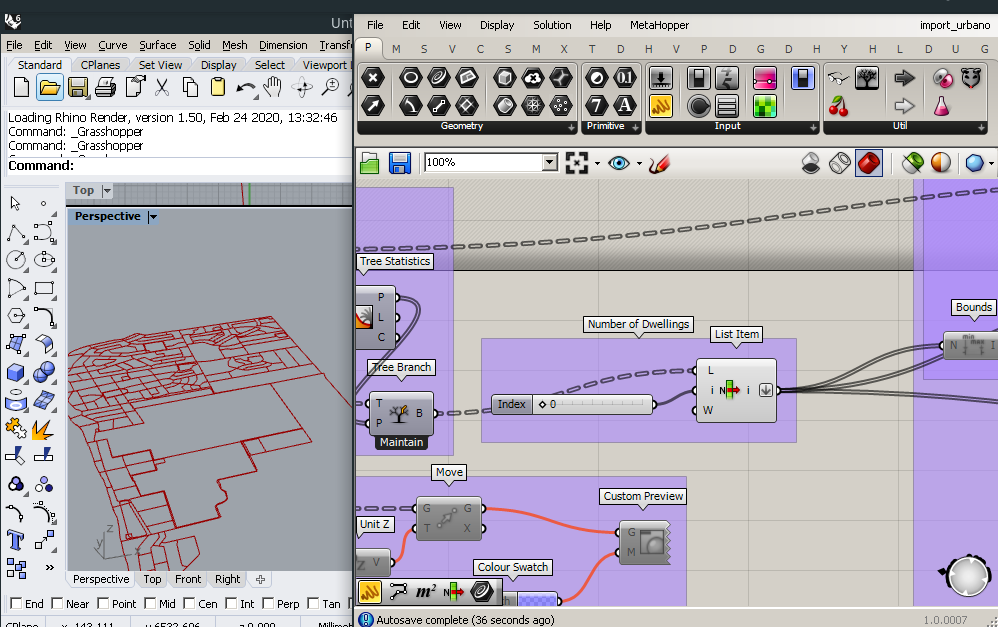
Then we need to clean the values and geometries that become invalid during the clipping process. First, we Flatten the Polylineoutput which are organised in branches, then we restructure the data tree using Graftcomponent, isolating each polyline geometry in a different list. Then, we use Clean Tree component to clean the invalid geometry, including empty branches. Clean tree component is located underSet > Tree > Clean Tree. Then, we use the component Tree statistics to extract all the branches names with valid geometry to use as a reference for the output Values from the Deconstruct Metadata component. Finally, we use the Tree Branch component to select the valid features that match the valid polylines. The output Pathsfrom Tree statistics in the input Path of Tree Branch and the output Values from Deconstruct Metadata in the input Tree of Tree Branch. Now our data is cleaned to be manipulated.
So, the process to import shapefiles in Grasshopper finished, then we can start to manipulate the data to generate or extract the information that we want.
For example, we can extract the number of dwelling that for each polyline that we have using the index 0 of a List Item component.
Then we can use that information to generating a gradient map based on the number of dwellings for each polyline.
To do that we can extract the high and low number in our list as a domain with the component Bounds which is located under Maths > Domain > Bounds before we connect our list in the bounds we need to Flatten the branches in a single list. Then, we deconstruct this domain using the component Deconstruct Domainlocated under Maths > Domain > Deconstruct Domain. We are going to use the Gradientcomponent to build our gradient map, it is located under Params > Input > Gradient. Right-click in the Gradientcomponent and Presets to choose the colour pattern to Red to BLue. It is important to notice that the pattern will be inverted to match the highest value in red and the lowest value in blue.so to do that we need to connect our Ènd output value from Deconstruct Domain in the Lower Limitvalue of the Gradient component and the Start output value from Deconstruct Domain in the Upper Limit value of the Gradient, then we connect our flattened list of values in the Parameter value of the Gradient. So, we have already built our gradient map based on the number of dwellings.
Then we can create a legend for our gradient map using Legend Settings located under Extreme Territories > Display > Legend Settings. This component ask for a Legend Origin as a Point3d, the Legend_Size_x and Legend_Size_Y which is related to the X and Y direction of the Legend Frame, an angle for rotate the legend Angle_Rotation_Legend (degrees), an offset for the title of the legend Legend_Offset, the Gradient Values, the Gradient Domain, the desired number of divisions that your legend will represent Number_of_divisions, and which kind of number representation the legend will have Domain Int (True) / Float (False), which can be in Integer (True) or Float (False) as a boolean condition.
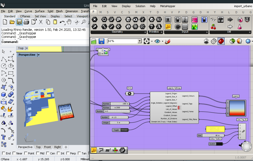
Finally, we can start to play with the other shapefiles. for example, we can move Greenspaces and Street Network in the Z direction, displacing it into space. To do that we can use the component Move component combined with Unit Z component and a Number Slider with an interactive numeric value for the translation. We can also combine it with Math operations, such as Multiplication to parametrically relate the two geometries. Finally, we can use the component Custom Preview and Colour Swatchto change the colours of our geometries.
So, we have finished our first tutorial on how to import shapefiles in Grasshopper using Urbano. The Grasshopper definition of this tutorial can be downloaded here, and the GIS files you can download here