Image Sampler + Planting
In this tutorial, we are going to explore how to populate a mesh geometry with trees based on an image. This grasshopper definition is a well-known method called Image Sampler, in which we can use an image as an input, extracting the pixels as points in a bidimensional plane as well as its features, such as saturation, colour, alpha channel, etc as input data that can generate or modify our grasshopper parameters. Image Sampler is a general approach that we can use in different circumstances as we can see in those examples. However, in this tutorial, we are going to use the image sampler method to populate with trees the terrain from the previous tutorial. We assume that you already have finished the tutorial “How to import a DTM file using Grasshopper / Docofossor”.
Therefore, this tutorial is divided into three parts:
- Preparing the image for Grasshopper
- Image sampler definition
- Populate the mesh with trees
1. Preparing the image for Grasshopper
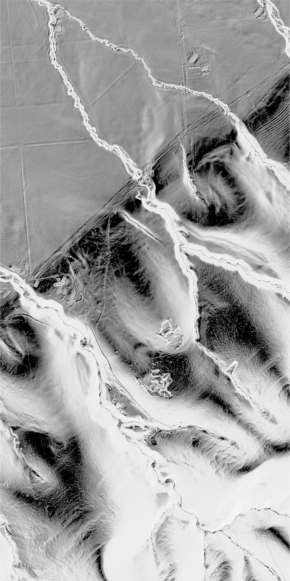
The first step in this tutorial is the preparation of the image that we will import into Grasshopper. In this tutorial we are going to use an image exported from Rhino that is the render preview of the terrain mesh that we have imported on the previous tutorial. First of all, we get the component Custom Preview. Go to Display > Preview > Custom Preview and then use the component Colour Swatch to choose a colour that highlight the topography, such as black.
After that, inside Rhino, we change the Rhino Viewport to Top view, and then we adjust it to fit into the size of the terrain. Next step is to export this visualisation as an image using the Rhino command ViewportCapturetoFile. Save it as .png, with transparency. Also, use viewport size with a scale factor that is close to the original size of our tiles 1000 x 2000.
Now we are going to open that image in a raster graphics editing software, such as Adobe Photoshop. In this tutorial I am using Gimp, which is an open-source alternative to Adobe Photoshop. However, you can use any similar software to do that task. First, we crop the image fitting the edges of the terrain.
Second, we resize the image to match the terrain tile 1000 x 2000pixels.
Then we duplicate the layer and overlay it with a multiply option. Also, we create a transparent layer.
So, now we are going to highlight the whiter part of our terrain ( We can imagine that the whiter part represents an analysis, information of the terrain, a sketch or other important information that you want to use as input in Grasshopper). We can highlight it even more if we invert the colours of the image, make them black.
In that case we are using a render image from Rhino, however, this process can be done with other kind of images that looking for other results, such as slope analysis, seasonal images, sketches, etc. The image will depend on the purpose that we are looking for.
2. Image sampler definition
First of all, we drop bifocals component on Grasshopper canvas, then we are going to define the boundary of the image with a rectangle component. Go to Curve > Primitive > Rectangle, then the input X we set as 1000 and the Y as 2000, which matches the size of our tile image.

Now, we create a mesh plane with the number of faces matching the number of pixels of the image. Go to Mesh > Primitive > Mesh Plane. Connect the X value from the same parameter of the rectangle in the input W(Width) of the Mesh Planecomponent and repeat the same process for the Y connecting into the H(Height) of the Mesh Plane.
However, we can not visualise the faces of the mesh because the option for display it is off by default. If you want to visualise the faces we can do that by going to Grasshopper menu Display > Preview Mesh Edges or using the shortcut Ctrl + M. For now, we are going to maintain the display off for do not overload our display card with unnecessary visualisations.
Now we are going to get the center of each face mesh using Face Normals component (for more information about the composition of a mesh geometry check here. Go to Mesh > Analysis > Face Normals, then connect the output M(Mesh) from Mesh Plane component into M(Mesh) input of Face Normals component.

Now it is time to sample our image using the Image Sampler component. Go to Parameters > Input > Image Sampler and drop the component into Grasshopper canvas. We are going to connect the output C(Center) from Face Normalscomponent into it. What it does is match pixels into points, returning pixel features, such as colour, saturation, alpha channel, etc that are going to be associated to X and Y coordinates of the mesh’s faces. We need to configure it component for it matches right. To do that, double click on Image Sampler component and then adjust the domain of X and Y to match the size of our image, which are in that case the domain for X go from 0 to 1000 and for Ygoes from 0 to 2000. After that, we click on ... to choose the image. By default, the image sampler will return colour values in RGB format. So, we are going to change it for Colour Brightness, in which the value is represented on a domain that goes from 0 to 1, from absolute black 0 to absolute white 1.
So, we can use a logical operator to filter the values that we are interested in. For example, if we want to get the values that are close to black we can use the logical operator Smaller than and set it to a value close to 0 for example 0.001. The component Smaller Than returns a True or False value. We can combine those results with the component Cull Pattern which filters a list based on a pattern defined by boolean values (True or False). It will get all values that are bellow to 0.001.
3. Populate the mesh with trees
In this part, we are going start to create the logic for populating our geometry with trees. The first step we need to define how many trees we want to spread through the sampled area. To do that we can use the Random Reduce component, which receive as inputs: the List L, the number of items to remove from the list R and the seed S which swap randomly the chosen elements to remove. So, if we want to know how many trees we need to remove to stay with the number of trees that we want to plant, we first need to count how many points we currently have on the area, then subtract by a number of trees that we want to plant. To do that we use the component List Lenght located on Set > List > List Lenght to the length of the list, then Subtraction component under Math > Operators > Subtraction. For example, if we want to plant 3000 trees, we subtract 3000 from the List Lenght output. After that, we connect the output L(list) from Cull Pattern component into input L(list) from Random Reduce component, then the output from Subtraction component into input R (number to reduce) of Random Reduce component. Finally, we put a number to control the S (seed) of our possibilities of distributions.
Now we need to project the points onto our mesh geometry. We can use the component Mesh Ray, which creates an infinite line that intersects a mesh based on points and a direction (vector). Currently, the points are bidimensional with a Z position equal 0, therefore the direction to project it onto our terrain is to up, or in the positive Z vector. First, we turn on the visualisation of the mesh terrain. Then, we get the component Mesh | Ray under Intersect > Mathematical > Mesh | Ray. We connect the mesh output from docofossor Grid Mesh component into input M(Mesh) of the component Mesh | Ray and the component Unit Z under the table Vector > Vector > Unit Z into the input D (direction) of the component Mesh | Ray. Finally, we connect the points from Random Reduce into input P of Mesh | Ray component. It will project our point on the top of the mesh terrain.
Now we need to create our trees based on those points. It will depend of the type of plant that we are going to choose to plant, however, in this tutorial we are going to see the logic of how to do, it will be based on a more generic approach, then, when you do that on your project you can adapt to your needs. So, we can create the tree stems following a vector in a Z direction. To do that we can use the component Line SDL located on Curve > Primitive > Line SDL. It will ask for a line length, the start points, and the direction for the line. So, to make it a little more dynamic we can use a random length for the tree stems based on a defined range. For example, we can say that our trees will have steam that may vary within a domain between 3 and 8 and then create random values that match the number of trees that we want. To do that we need to use the Random component. Go to Set > Sequence > Random we also will need the List Lenght component that we have already used before here. Besides that, we are going to create a specific domain for our tree steams, as I said, can vary within 3 and 8. To create the domain we are going to use the Construct Domain component under Math > Domain > Construct Domain.
We are almost finishing, now we just need to create the tree canopies. To do that we can create a simple visualisation with a Mesh Sphere, but first, we need to get the endpoints of those lines. To do that we can use the End Pointcomponent under Curve > Analysis > End Point which will return to us start and endpoints of those lines. For the radius of those spheres, we can create a simple parametric relation with each tree stem length, for example, we can divide the length of the tree stems by 2 or 3 and using the resulting value as the radius of the spheres. Connect the output of Line SDL component into the input of End Point component, then use the output from Random component into input A from Division component located under Math > Operators > Division. Use a number slider with 2 or 3 as value to divide that list into B input of Division component, these values go on the input R of the Mesh Sphere component. To make the visualisation process faster we can put a low value for sphere faces, such as 3, this value goes in inputs U and V of the Mesh Sphere component. The location for the sphere will be the endpoints from the output E from the component End Point. For visualisation purpose, we can use a Custom Preview and Colour Swatch components.
The final touch that we can do is change the colour of the mesh terrain.
We have finished this tutorial. You can download the Grasshopper file here and the image used on image sampler here.